The Magic of Naming Cells in Excel

Why Naming Cells in Excel is beneficial?

Naming cells in Excel makes life easier in many cases. For example, It helps when you use a complex financial model with lots of data and sheets. You would rather remember “profits” instead of the cell value that contains the value of the profits.

By naming cells or cells ranges in Excel you can quickly jump to the relative cell, or use it in the formula without actually getting to the cell.

What are the rules of naming cells/ranges in Excel?

When creating named cells/ranges, follow these rules:

1. Begin with a letter, an underscore (_), or a backslash (\).
2. Names can’t contain spaces and most punctuation characters.
3. You can’t conflict the names with cell references – you can’t name a range “A1” or “Z100”.
4. Single letters are OK for names (“a”, “b”, “c”, etc.), but the letters “r” and “c” are reserved. Names are not case-sensitive – “home”, “HOME”, and “HoMe” are all the same to Excel.

What is an example of naming cells in Excel?

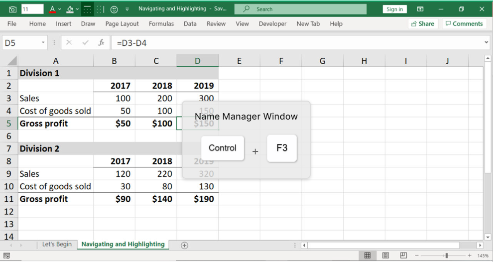
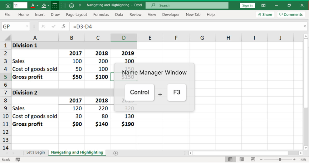
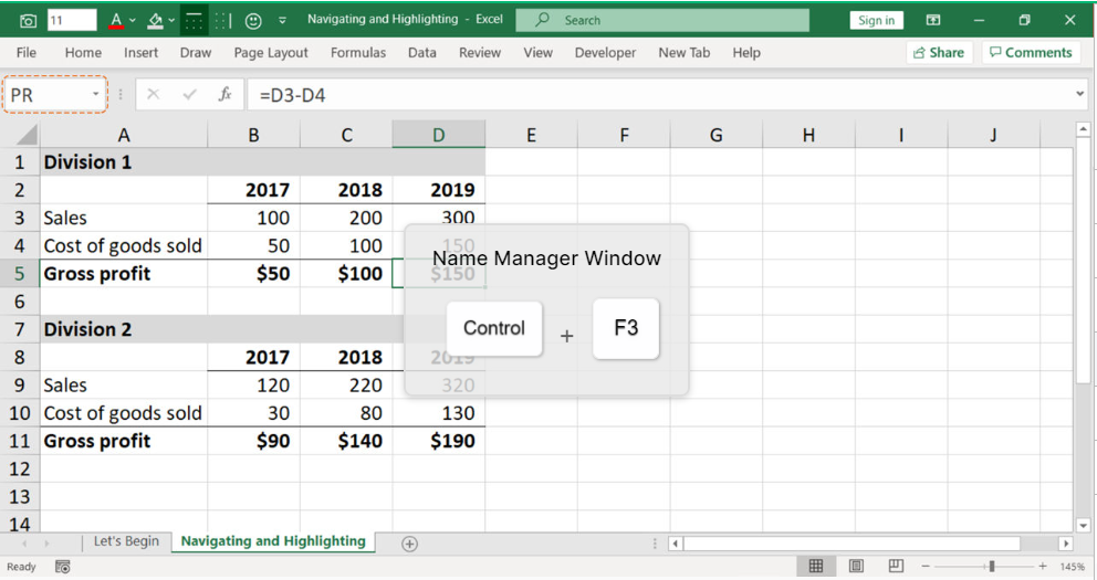
To name a cell in Excel, use the Name Manager window. Excel shortcut Ctrl + F3 will open this window for you.

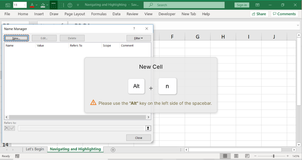
After you open the “Name Manager” window, you can create a new name by clicking the button “New” or using shortcut Alt + N (Alt and underlined letter).

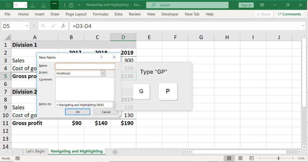
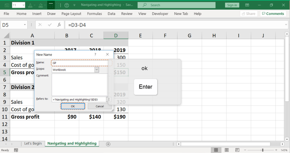
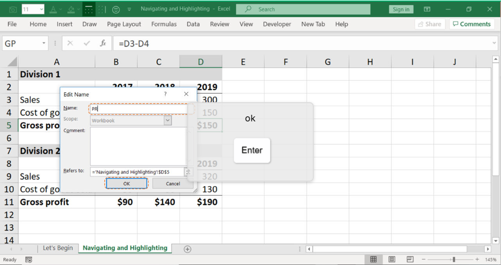
Let’s name our cell “GP” for our example. Then click “Enter” or “OK” to apply.

Click Esc to close the window.

You can see in the top left corner of the picture below that the cell’s name is “GP” now. Let’s see how easy it is to navigate to this cell now, no matter where in the spreadsheet you are. Let’s go to the cell A1 by using Excel shortcut Ctrl + Home.

Now when we are in the cell A1 and want to get to the cell named “GP” quickly, let’s use “Go To” window in Excel. You can open that window with the shortcut F5.

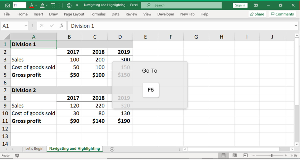
In the “Go To” window in the “Reference” field type the name of the cell you would like to jump to. In our example, it’s “GP”.

Great, you jumped to the named cell in a couple of clicks. Now, let’s edit the name. For that let’s open the “Name Manager” window again with Ctrl + F3 shortcut.

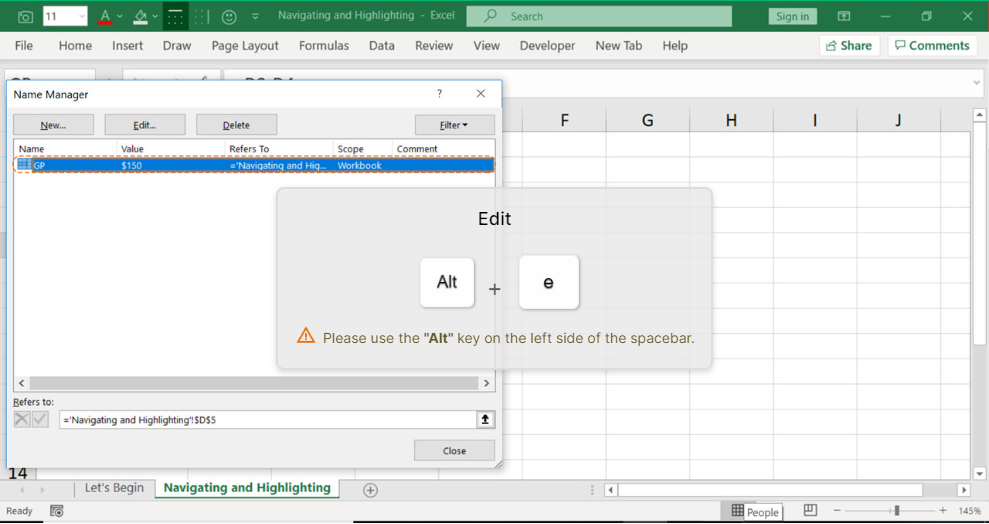
Let’s edit the named cell by clicking the button “Edit” or using shortcut Alt + E (Alt and underlined letter).

How to change the cell names?

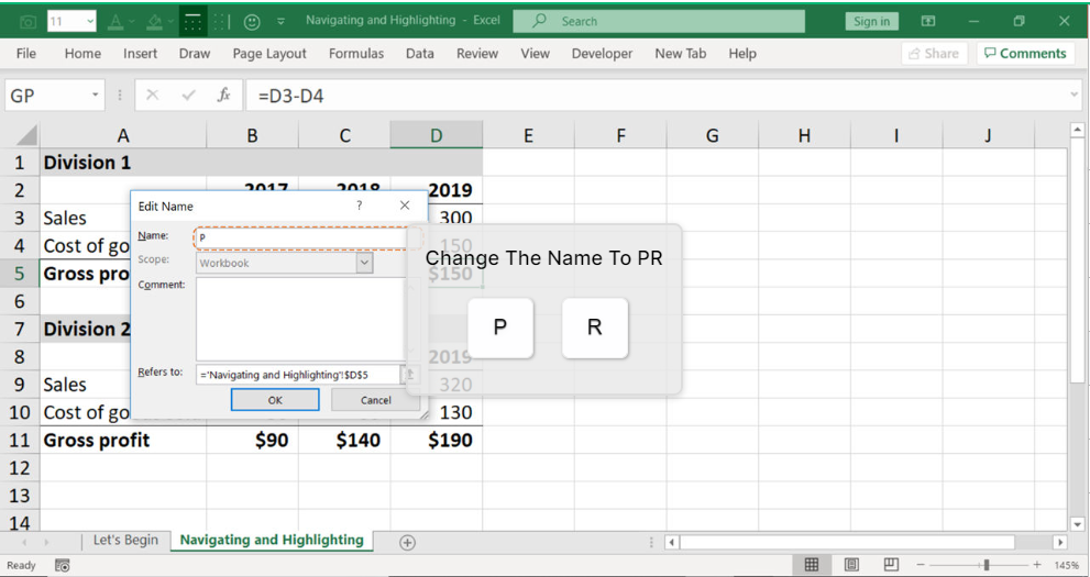
Let’s change the name from “GP” to “PR”.

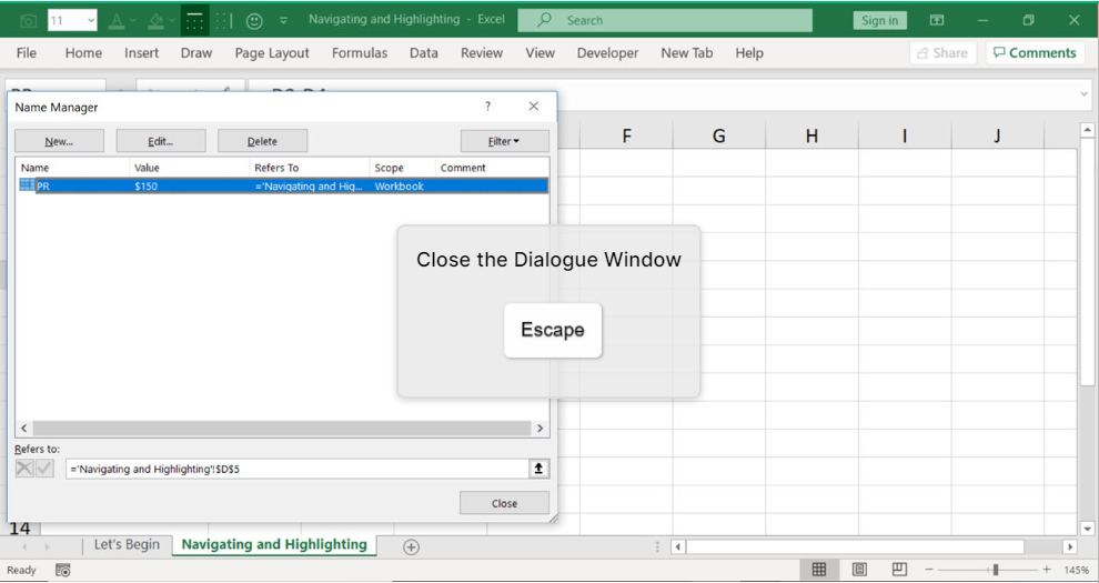
After editing is done, click Esc to close the “Name Manager” window.

You can see in the top left corner of the picture below that the cell is named “PR” now. Now, let’s delete the name. For that let’s open the “Name Manager” window again with Ctrl + F3 shortcut.

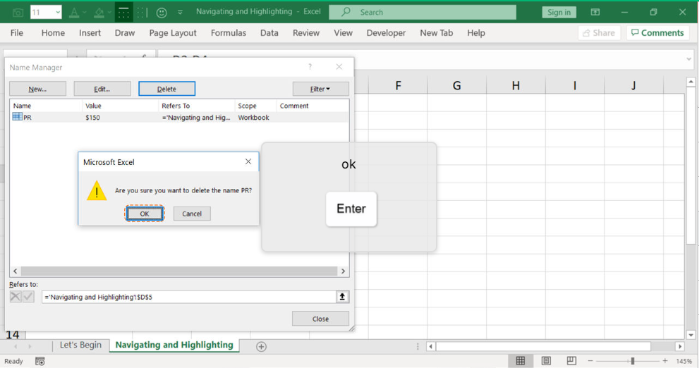
To delete the named cells click the button “Delete” or using shortcut Alt + D (Alt and underlined letter).

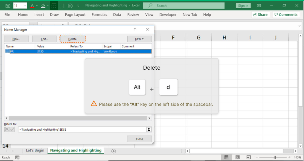
Click “Enter” or “OK” to confirm the action.

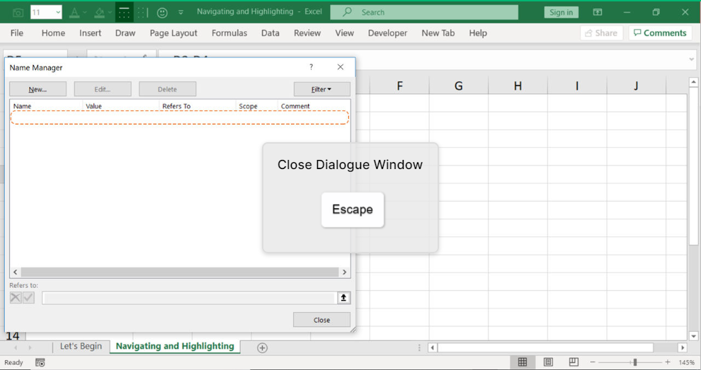
Close the dialog window with Esc.

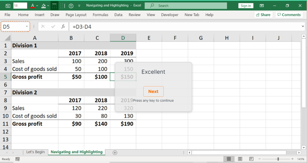
You can see in the top left corner of the picture below that the cell does not have the name anymore as we have deleted it, now it’s just “D5” in the field.

Following the same logic as creating a name for a cell, you create a name for cells ranges.

You can also use named cells/ranges in the formulas. They can make formulas a lot easier to create, read, and maintain. And as a bonus, they make formulas easier to reuse (more portable).

Conclusion

Naming the cells/ranges is one of the Excel tricks that can help you to speed up your workflow in Excel and accomplish tasks much quicker. Learn more Excel tricks by playing our educational games keySkillset.

‍