Why do we use anchoring in financial models?
In this article, we will discuss the anchoring in financial models in Excel and see how this formula can help you to reduce a significant amount of your time working on your Excel files.
Anchoring is probably the most used shortcut in Excel. By pressing F4, you can select different options for anchoring. It means locking the cells inside the formulas from different dimensions. Let’s look at the examples below to see how the anchoring option works in financial modeling.
How to use anchoring for projections?
In our model, we assume that revenue growth in 2019 is 14.3% and then it goes down each projected year by 0.5%. Instead of just using (0.5%) in the formula, we have created a cell with the step (K27).
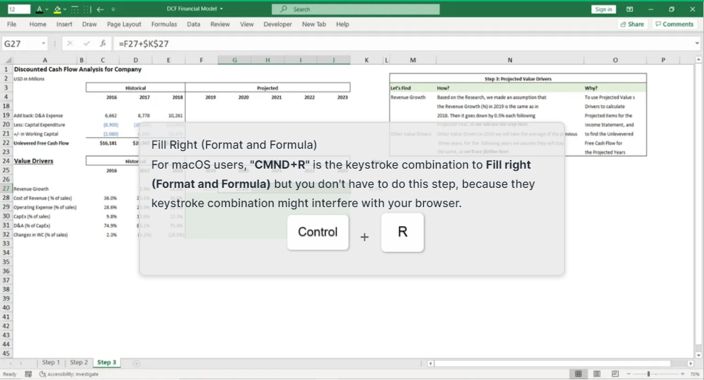
Our formula is written on the picture below and it is correct for the cell G27. We would like to fill that formula to the right for the cells H27 – J27. For that we need to anchor $K$27, so we can fill the formula to the right freely with keeping the correct formula for all projected years.
If we do not anchor the cell K27, then in H27 the formula would move K27 to the right and apply L27, which would be incorrect for our purpose.
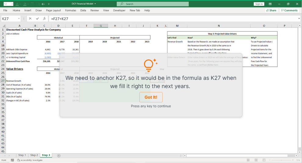
Let’s anchor the cell with F4 Excel shortcut.
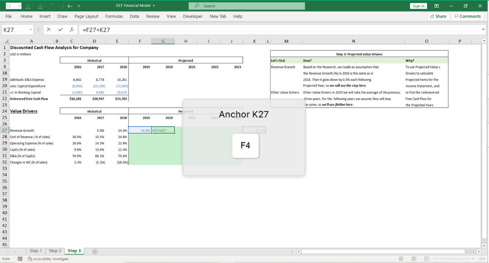
F4 is a toggle and you can anchor differently by clicking F4 several times:
- you can anchor both column and row,
- then, anchor only column,
- anchor only row
- get rid of anchoring.
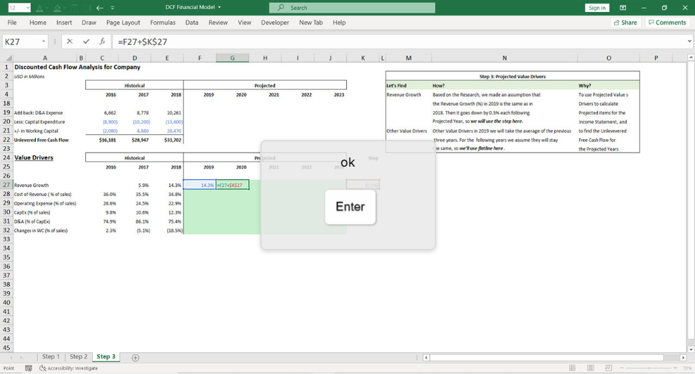
In our example a total anchoring of the row and the column works perfectly. Let’s click “Enter” to apply the correct formula.
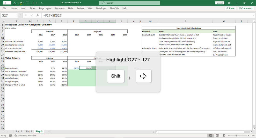
Now we can easily fill formula with the anchored cell to the right and be sure it will be correct:
- Shift + Right Arrow to highlight G27 – J27,
- Ctrl + R to fill right.

Conclusion
You can learn more about anchoring formula in Excel in our article “Anchoring Formula in Excel”.
Learn more Excel functions and speed up your Excel workflow and Financial Modeling skills by playing our educational games keySkillset.


.jpg)
.jpg)


.jpg)
.jpg)


.png)

