

Are you tired of spending hours trying to figure out complicated calculations in Excel? Well, you're in luck! Excel has an entire library of functions that can make your life a whole lot easier.
In this post, we will explore some of the most common basic functions in Excel, including how to use them, why they are important, and alternative suggestions to help you streamline your calculations.
Here are some basic Excel functions that you have to work with:
1.AutoSum Function
Excel can easily calculate the sum of a row or column of numbers for you. By using the AutoSum feature, you can save time and avoid the potential for manual errors in your calculations.
How to use it:
Select the cell where you want to display the sum of the data. This cell should be located directly below the column of data you want to sum or directly to the right of the row of data you want to sum.
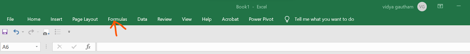
Go to the Formulas tab in the Excel Ribbon.
Click on the "AutoSum" button in the Formulas group. The AutoSum button looks like a Greek letter Sigma (∑).

Excel will automatically select what it thinks is the range of cells that you want to sum. Check to make sure that the range is correct.
If Excel has not correctly selected the range of cells to sum, drag your mouse over the cells you want to sum to highlight them. Excel will automatically adjust the formula based on the new selection.
Press "Enter" to complete the AutoSum calculation. Excel will add up the numbers in the selected range and display the total in the cell where you entered the formula.
Example:
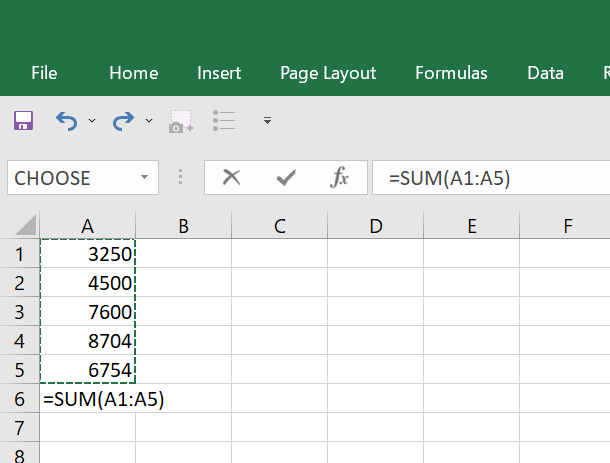
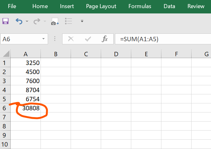
As you can see from the screenshot above, if you want to add up the values in cells A1 to A5, the formula would be "=SUM(A1:A5)" and the result you get is:
Alternative suggestions:
- Using the keyboard shortcut: Select the cell where you want the result to appear, and press "Alt" + "=" on your keyboard. Excel will automatically select what it thinks is the range you want to add up, and you can hit enter to confirm.
2. Calculate MEAN in Excel using AVERAGE formula
Calculating the mean of numbers is one of staples of statistical analysis processes. In this article, we're going to show you how to calculate mean in Excel using the AVERAGE formula. The mean, also known as the statistical average, is the central value of a set of data and is calculated by adding up all the data points and dividing the total by the number of points. Excel's AVERAGE function follows this same principle by summing up all the values and then dividing the total by the count of numbers in the set.
How to use it:
The AVERAGE function takes a range of cells as its argument and returns the average of those cells. Select the cell where you want the result to appear.
Type "=AVERAGE(" followed by the range of cells you want to find the average for, separated by commas.
Close the parentheses and hit enter.
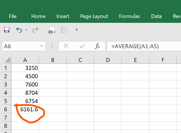
Example:
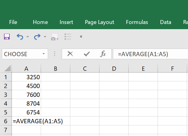
As you can see if you want to find the average of the values in cells A1 to A5, the formula would be "=AVERAGE(A1:A5)". So the result is:
3. COUNT Function
The COUNT function counts the number of cells in a range that contain numbers. It's useful when you want to count the number of values in a dataset.
How to use it:
Select the cell where you want the result to appear.
Type "=COUNT(" followed by the range of cells you want to count, separated by commas.
Close the parentheses and hit enter.

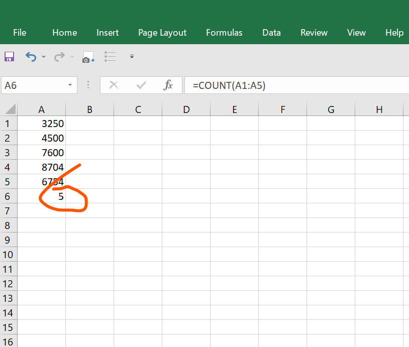
Example:
Now, in the screenshot above you can see that if you want to count the number of cells that contain numbers in cells A1 to A5, the formula would be "=COUNT(A1:A5)". As you can see the result is the no of cells that contain numbers:
Alternative suggestions:
You can use the COUNTA function to count the number of cells in a range that contain any value, including text or blank cells.
4. MAX Function
The MAX function returns the highest value in a range of cells. It's useful when you want to find the highest or maximum value in a dataset.
How to use it:
Select the cell where you want the result to appear.
Type "=MAX(" followed by the range of cells you want to find the maximum value for, separated by commas.
Close the parentheses and hit enter.
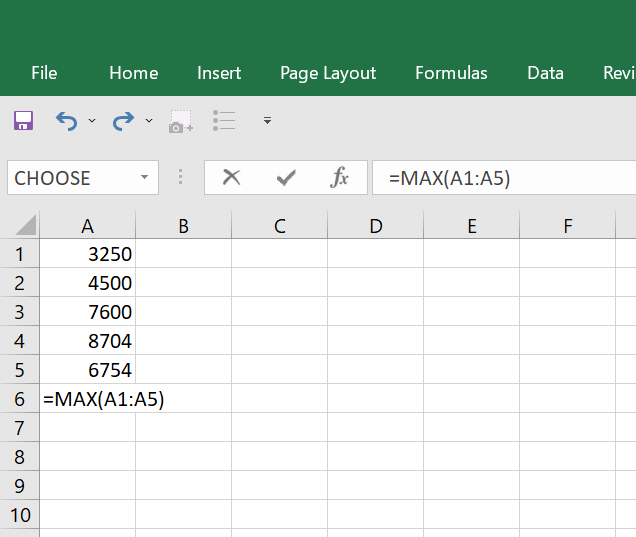
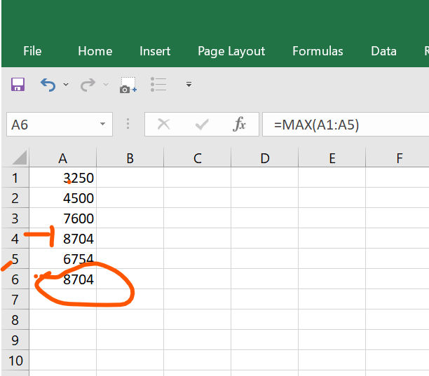
Example:
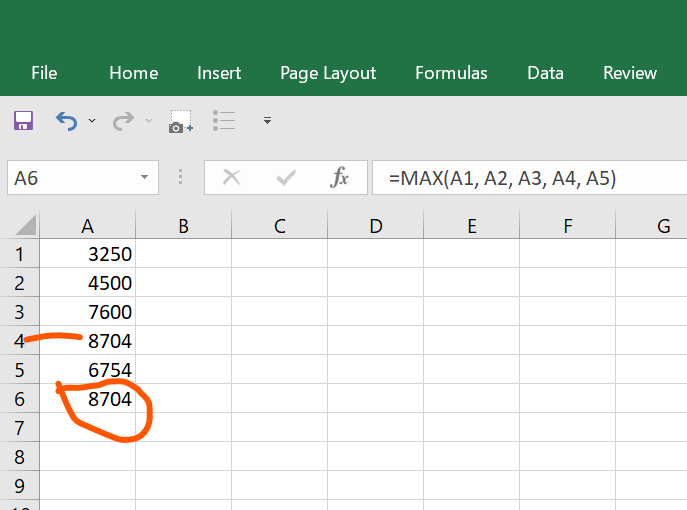
If you want to find the highest value in cells A1 to A5, the formula would be "=MAX(A1:A5)". And the result you get is given below:
Alternative suggestions:
There are a few alternative ways to use MAX Function:
- Using the "MAX" function with cell references: Instead of directly entering the cell range, you can use cell references within the MAX function. For example, "=MAX(A1, A2, A3, A4, A5)" would return the same result as "=MAX(A1:A5)".
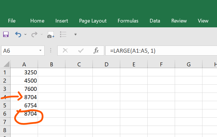
- Using the "LARGE" function: The LARGE function returns the nth largest value in a range. If you want to find the largest value, you can use the LARGE function with "n" set to 1. For example, "=LARGE(A1:A5, 1)" would return the same result as "=MAX(A1:A5)".
5. COUNTIF Function
The COUNTIF function is used to count the number of cells within a range that meet a specific criterion. For example, you can use the COUNTIF function to count the number of times a certain product was sold, or the number of employees who have more than 5 years of experience.
How to use it:
Select the cell where you want the result to appear.
Type the equals sign (=) followed by the COUNTIF function name.
Inside the parentheses, enter the range of cells you want to count, followed by a comma (,).
Enter the criteria you want to apply in quotation marks (""), followed by a closing parenthesis ().
Example:
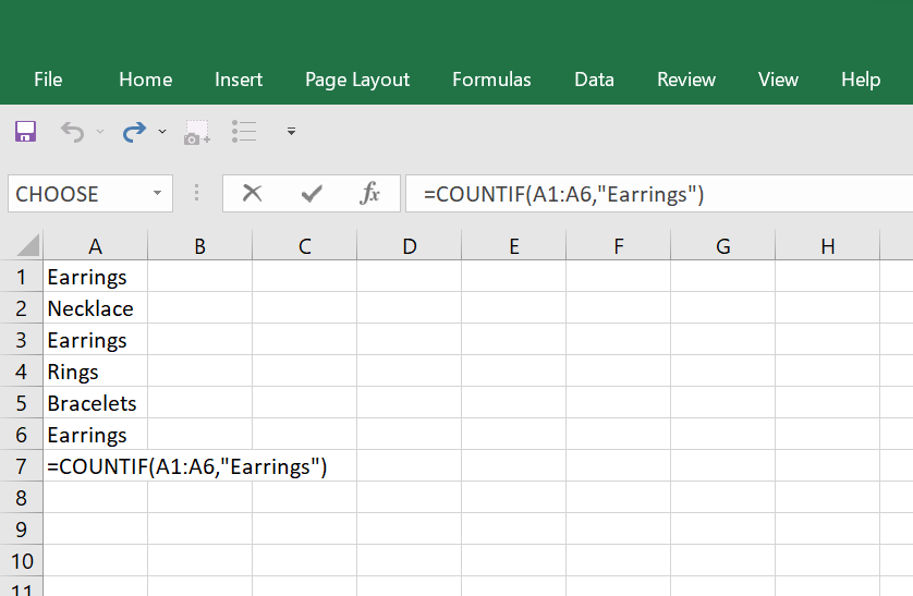
For example, to count the number of times "Product A" appears in cells A1 through A6, use the following formula:
=COUNTIF(A1:A6,"Product A")
This will return the number of times "Product A" appears in the specified range.
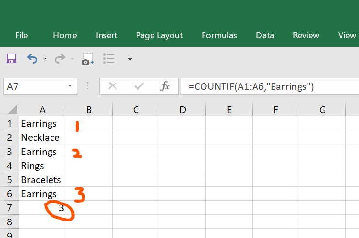
As you can see from the image above, the number of times "Earrings" appears in cells A1 through A6, is 3 so if we use the following formula: =COUNTIF(A1:A6,"Earrings.") The answer you get is:
Alternative suggestion:
- Using the SUMPRODUCT function: The SUMPRODUCT function can be used to count the number of times a criteria appears in a range. For example, "=SUMPRODUCT(--(A1:A6="Product A"))" would return the number of times "Product A" appears in the range A1:A6.
6. CONCATENATE Function
The CONCATENATE function is used to combine text strings from multiple cells into a single cell. For example, you can use the CONCATENATE function to combine a person's first name and last name into a single cell.
How to use it:
Select the cell where you want the result to appear.
Type the equals sign (=) followed by the CONCATENATE function name.
Inside the parentheses, enter the cells or text strings you want to combine, separated by commas.
Example:
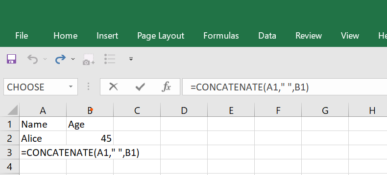
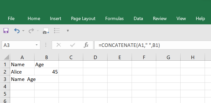
To combine the text in cells A1 and B1, use the following formula:
=CONCATENATE(A1," ",B1)
This will combine the text in cells A1 and B1, separated by a space. And the result is:
Alternative suggestion:
- Using the "&" operator: Instead of using the CONCATENATE function, you can use the "&" operator to join text strings together. For example, "=A1&B1" would concatenate the values in cells A1 and B1.
7. LEFT and RIGHT Functions
The LEFT and RIGHT functions are used to extract a specified number of characters from the left or right side of a cell.
How to use the LEFT Function in Excel:
Select the cell where you want the result to appear.
Type the equals sign (=) followed by the LEFT function name.
Inside the parentheses, enter the cell and the number of characters you want to extract, separated by a comma.
Example:
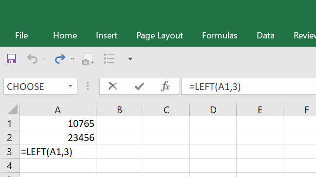
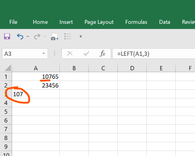
To extract the first 3 characters from cell A1, use the following formula:
=LEFT(A1,3)
This will extract the first 3 characters from cell A1.
How to use the RIGHT function in Excel:
Select the cell where you want the result to appear.
Type the equals sign (=) followed by the RIGHT function name.
Inside the parentheses, enter the cell and the number of characters you want to extract, separated by a comma.
Example:
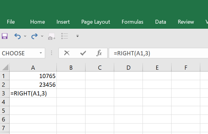
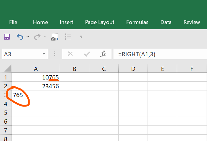
To extract the last 3 characters from cell A1, use the following formula:
=RIGHT(A1,3)
This will extract the last 3 characters from cell A1.
Alternative suggestion:
You can also use the MID function to extract characters from the middle of a cell.
Conclusion
Alternatively. Excel is a powerful tool that can help you organize and analyze your data quickly and efficiently. By mastering the basic functions in Excel, you can save time and improve your productivity. In this blog post, we covered a few of the basic functions in Excel: SUM, AVERAGE, MIN, MAX, COUNTIF, CONCATENATE, LEFT, and RIGHT. Remember to use these functions in combination with other Excel features like sorting, filtering, and conditional formatting to get the most out of your data.
Also, here is some information about our Excel Program. We have a simulation-based Excel Efficiency program on keySkillset.
.svg)

.svg)
Start learning new skills with the help of KeySkillset courses and our learning management system today!


keySkillset is a Learning Management System developed to make learning key business software skill sets easy through guided simulated learning.


